Unit 3 - Production, Cost, and the Perfect Competition Model
Table of Contents
3.1 - The Production Function
Key Terms & Definitions
The Production Function
The relationship between the quantity of inputs (factors of production) used to make a good and the quantity of output of that good.
- •Short Run: At least one input (usually capital) is fixed.
- •Long Run: All inputs are variable.
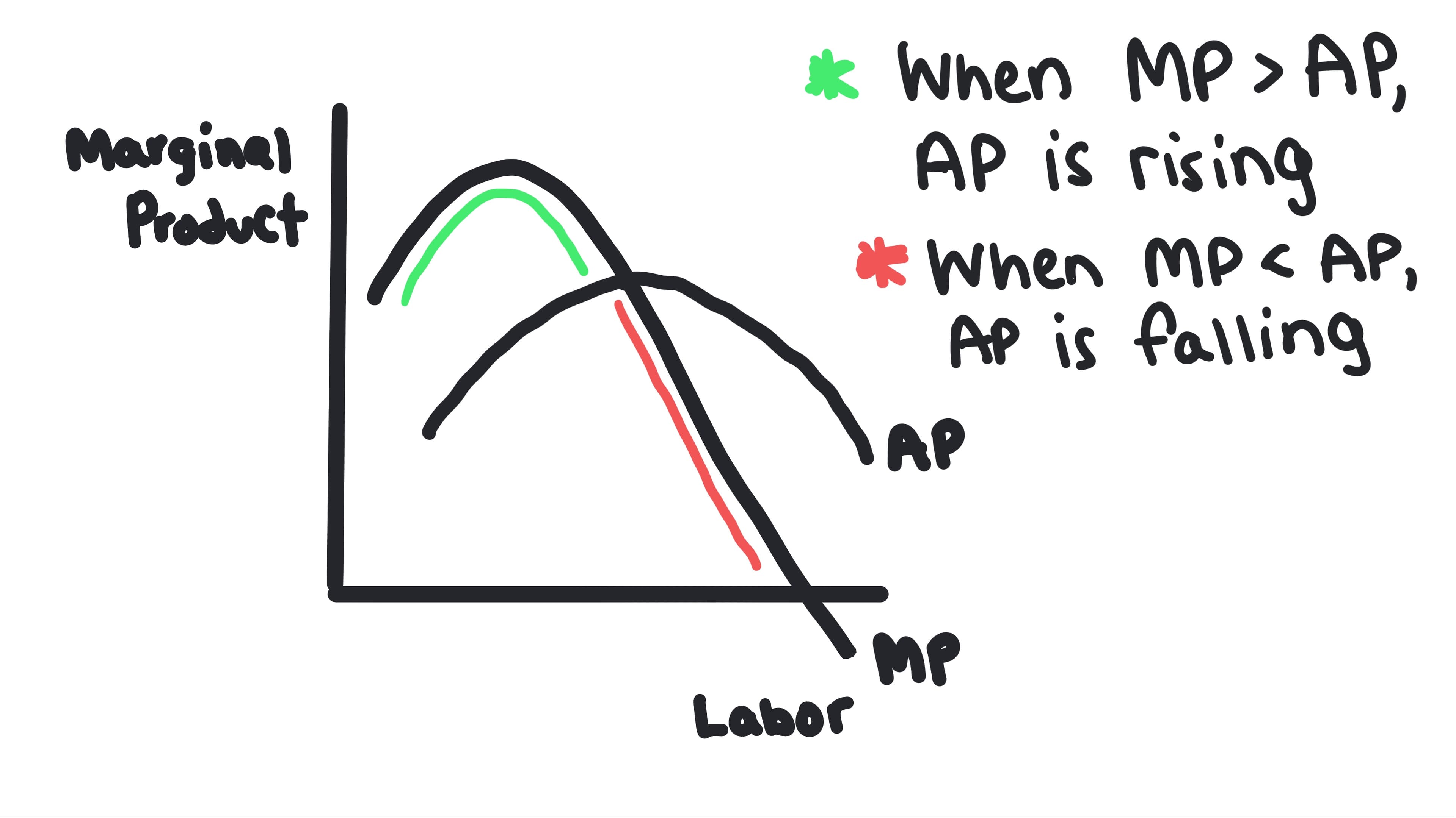
Marginal Product (MP)
The additional output produced by hiring one more unit of a variable input (like one more worker).
- •Formula: Change in Total Product / Change in Inputs
- •MP intersects Average Product (AP) at the maximum point of AP.
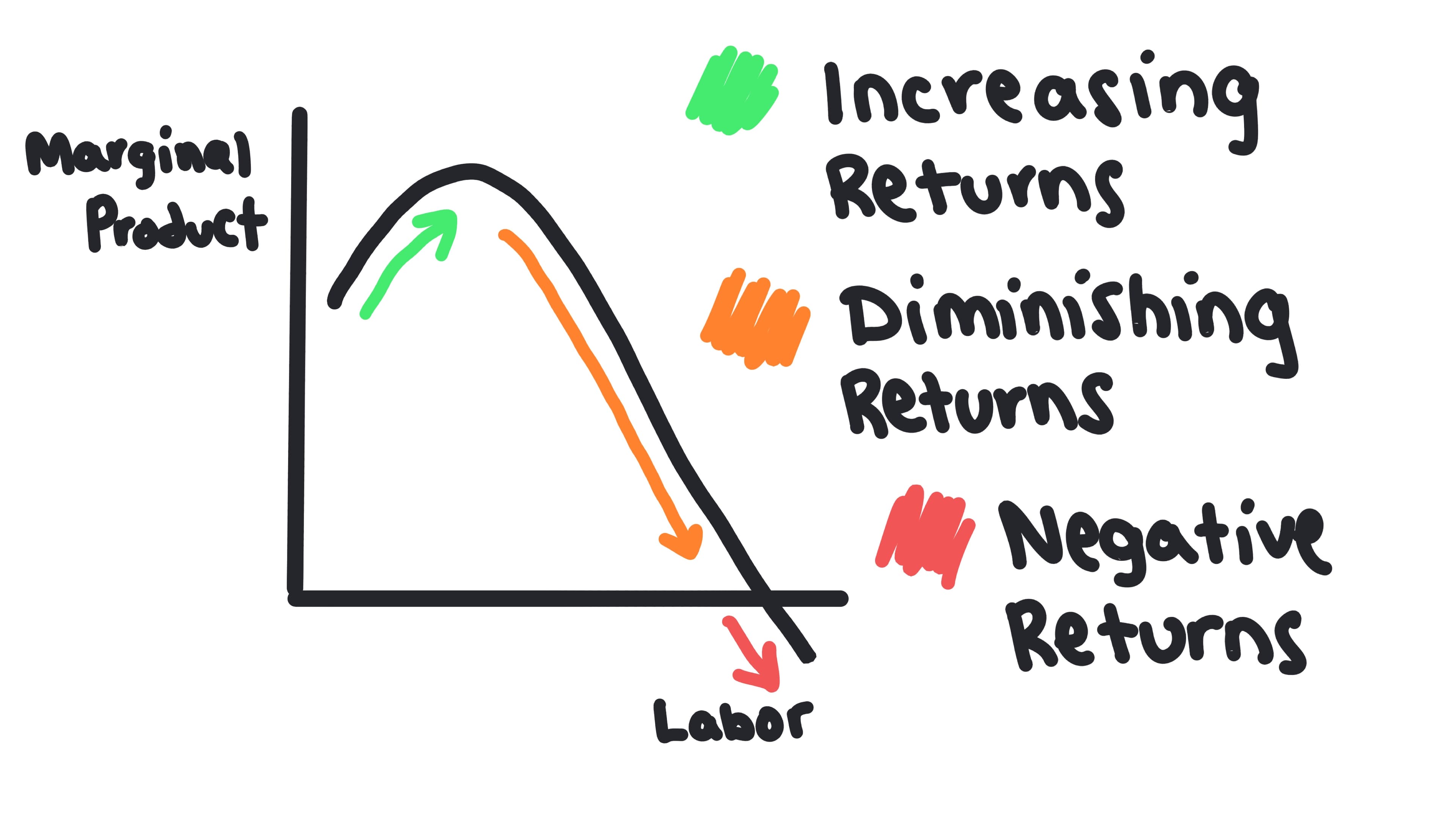
Law of Diminishing Marginal Returns
A principle stating that as more units of a variable input are added to a fixed input, the marginal product of the variable input will eventually decline.
- •Example: If you keep adding chefs to a kitchen with a fixed number of ovens, the marginal product of the chefs will eventually decline as they start to get in each other's way.
- •This explains why the Marginal Cost (MC) curve eventually slopes upward.
Whiteboards

3.2 - Short-Run Production Costs
Key Terms & Definitions
Fixed Costs
Costs that do not change with the level of output produced.
- •Remain constant regardless of production level
- •Example: Monthly rent for a factory, insurance premiums, or loan payments
- •Must be paid even if output is zero
Variable Costs
Costs that change with the level of output produced.
- •Increase as output increases, decrease as output decreases
- •Example: Wages for hourly workers, raw materials, electricity used in production
- •Zero when output is zero
Total Costs
The sum of all fixed costs and all variable costs at a given level of output.
- •Formula: Total Cost (TC) = Total Fixed Cost (TFC) + Total Variable Cost (TVC)
- •Example: If a factory has $10,000 in fixed costs (rent) and $5,000 in variable costs (materials and labor) for producing 100 units, total cost is $15,000
- •Increases as output increases due to variable costs
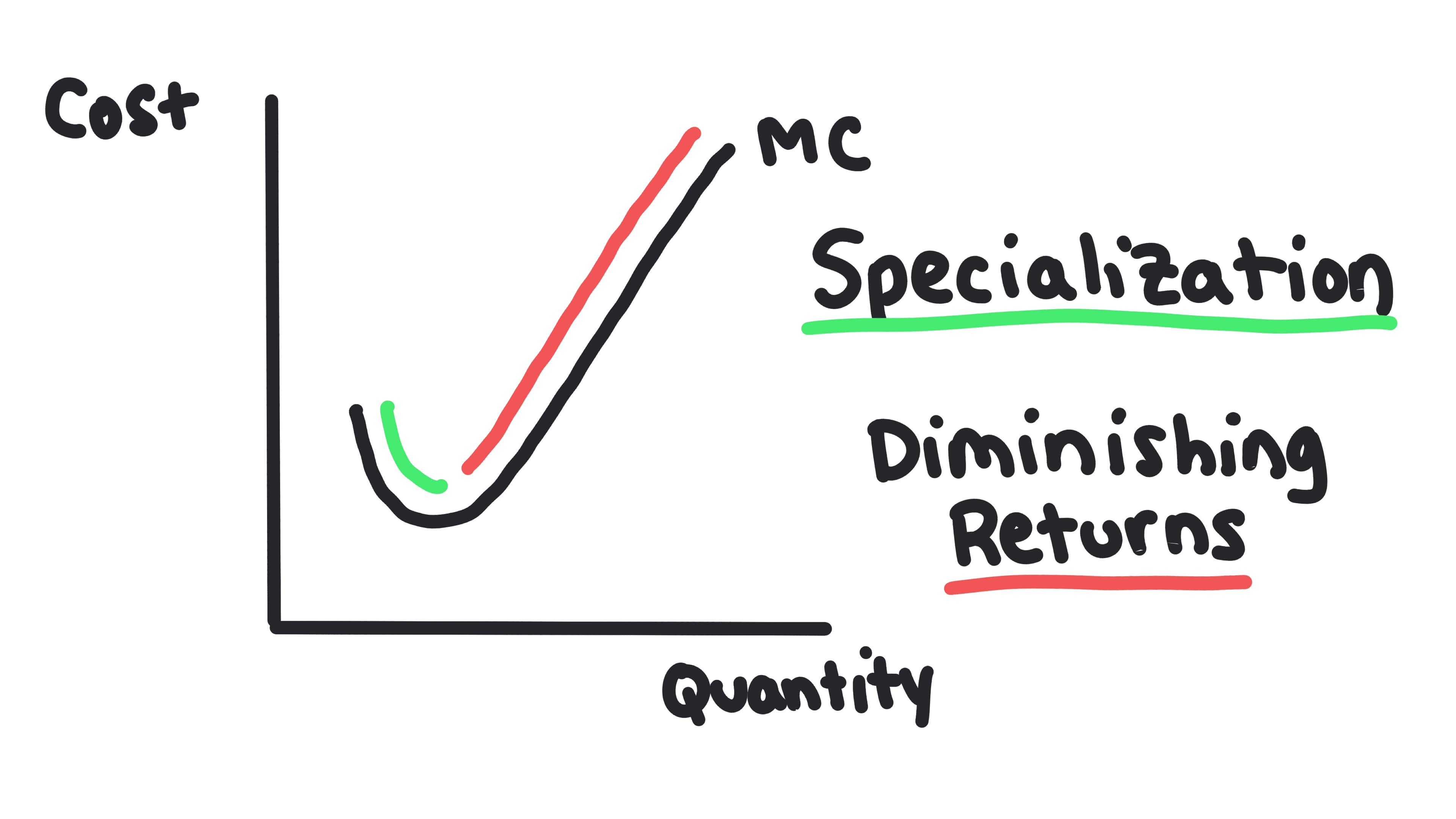
Marginal Cost (MC)
The additional cost incurred by producing one more unit of output.
- •Formula: Change in Total Cost / Change in Quantity
- •The MC curve looks like a Nike swoosh.
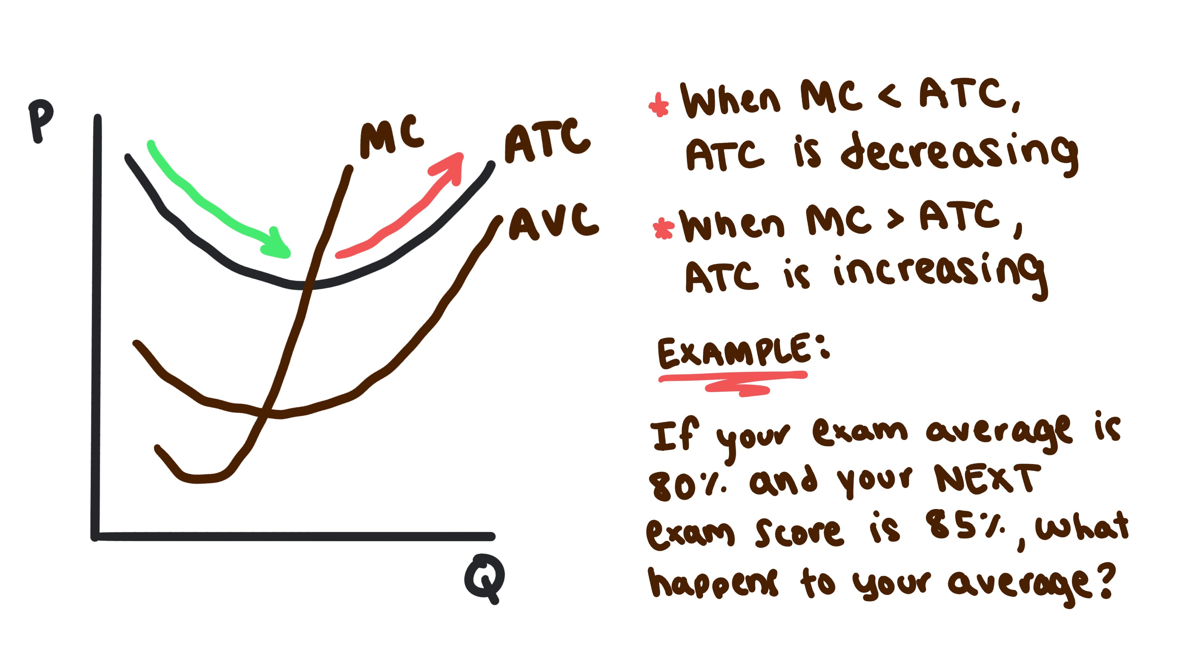
- •MC crosses ATC and AVC at their minimum points.
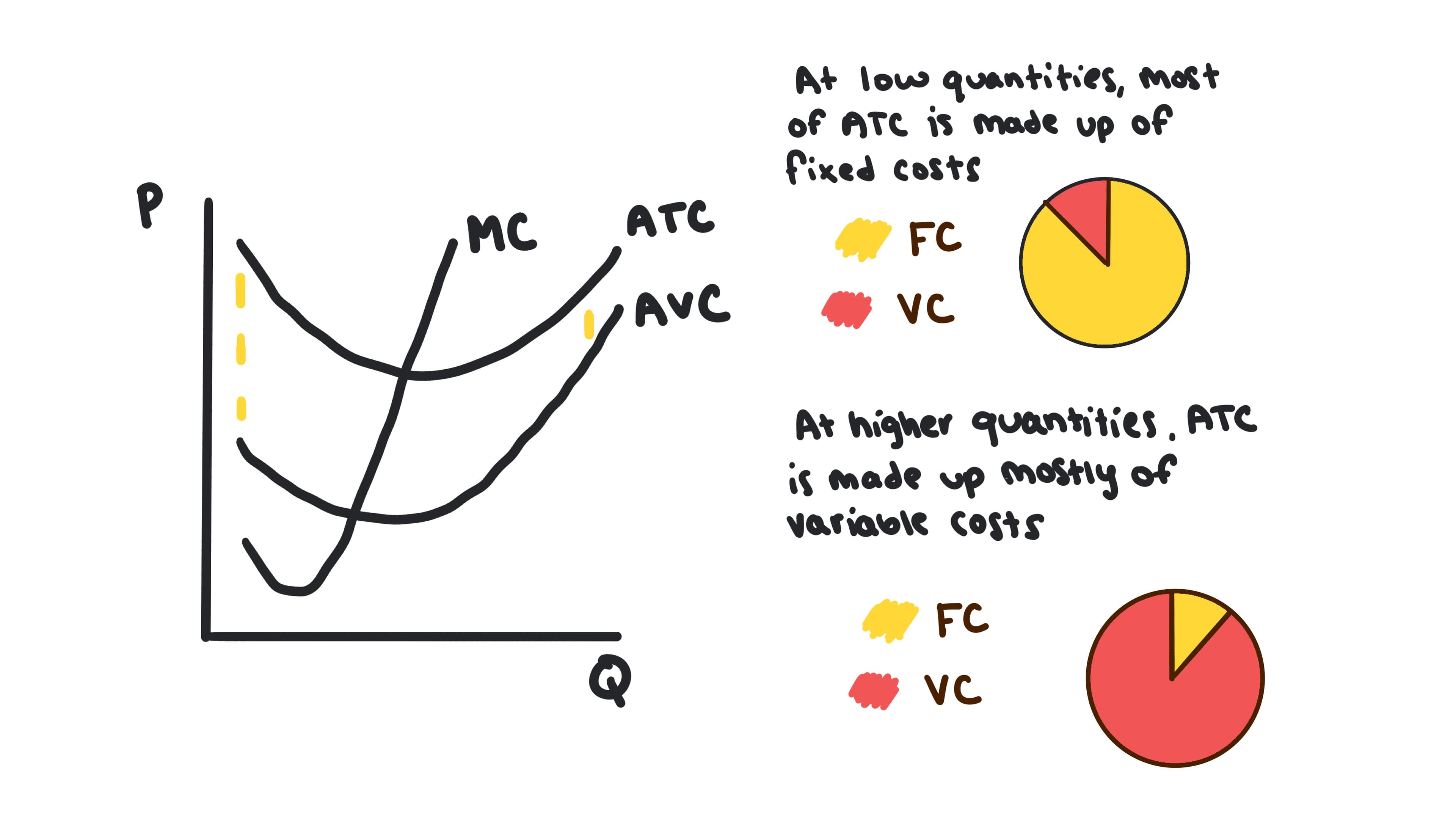
Average Total Cost (ATC)
The total cost divided by the quantity of output produced.
- •Formula: TC / Q or AFC + AVC
- •The curve is U-shaped due to economies of scale and diminishing returns.
Average Variable Cost (AVC)
The variable cost divided by the quantity of output produced.
- •Formula: TVC / Q
- •Gets closer to ATC as output increases because Average Fixed Cost (AFC) declines.
Whiteboards
3.3 - Long-Run Production Costs
Key Terms & Definitions
The Long Run
A time period in which all factors of production are variable; there are no fixed costs.
- •Firms can adjust all inputs, including plant size and capital.
- •All costs are variable in the long run.
- •Firms can enter or exit the industry in the long run.
Economies of Scale
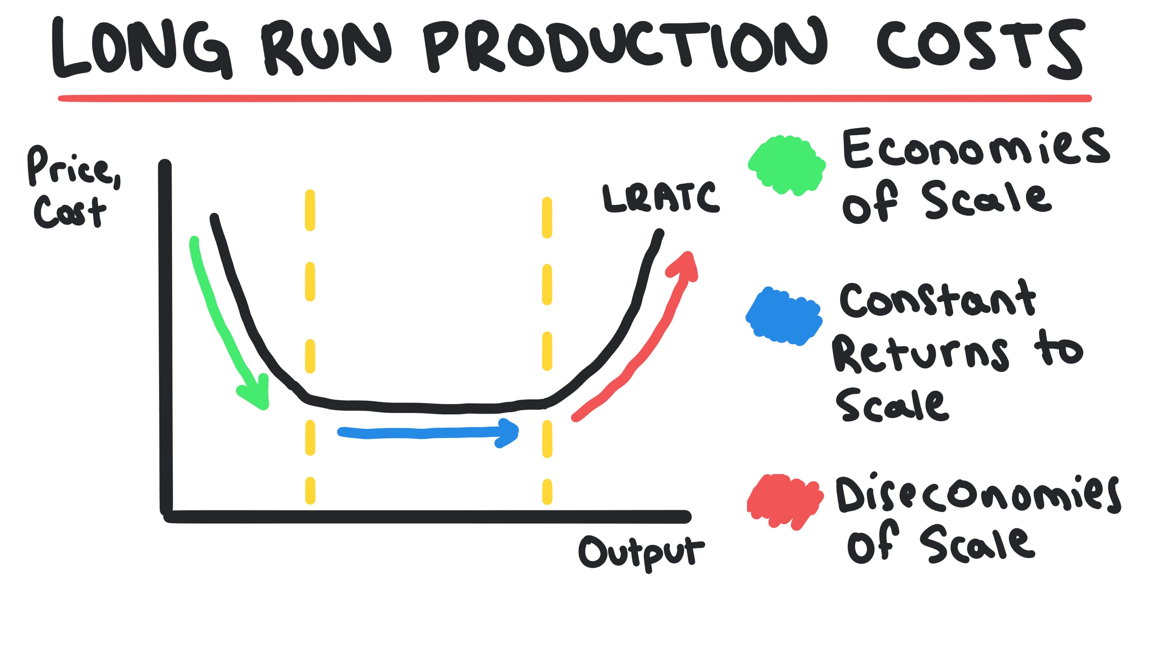
When long-run average total cost falls as the quantity of output increases.
- •Occurs due to specialization and bulk purchasing.
- •Represented by the downward-sloping portion of the LRATC curve.
- •Explains why large companies are often more efficient than small companies.
Diseconomies of Scale
When long-run average total cost rises as the quantity of output increases.
- •Occurs due to coordination problems and bureaucracy in very large firms.
- •Represented by the upward-sloping portion of the LRATC curve.
- •In other words, a company has become too big for its own good.
Whiteboards
3.4 - Types of Profit
Key Terms & Definitions
Explicit Costs
Direct, out-of-pocket payments for inputs.
- •These are clearly seen on a receipt.
- •Example: Wages for hourly workers, rent for a factory, materials for a product.
Implicit Costs
The opportunity costs of using resources that the firm or individual already owns.
- •These are not recorded in accounting books but are crucial for economic decisions.
- •Example: Salary that a business owner could have earned working for someone else.
Accounting Profit
Profit calculated by subtracting only explicit costs from total revenue. Does not consider implicit costs (opportunity costs).
- •Formula: Accounting Profit = Total Revenue - Explicit Costs
- •A firm can have positive accounting profit but zero economic profit.
Economic Profit
Profit calculated by subtracting both explicit costs and implicit costs (opportunity costs) from total revenue.
- •Formula: Economic Profit = Total Revenue - (Explicit Costs + Implicit Costs)
- •A firm can have positive accounting profit but zero economic profit.
Normal Profit
When economic profit is zero. This means the firm is covering all costs, including the opportunity cost of the owner's time and capital.
- •This is the long-run equilibrium condition for perfectly competitive firms.
Checkpoint
Test your understanding of 3.1
The law of diminishing marginal returns states that as more units of a variable input are added to a fixed input:
Checkpoint
Test your understanding of 3.2
Marginal Cost (MC) intersects Average Total Cost (ATC) at:
3.5 - Profit Maximization
Key Terms & Definitions
Marginal Cost (MC)
The additional cost incurred by producing one more unit of output.
- •Formula: Change in Total Cost / Change in Quantity
- •The MC curve looks like a Nike swoosh.
- •MC crosses ATC and AVC at their minimum points.
Marginal Revenue (MR)
The additional revenue generated from selling one more unit of output.
- •Formula: Change in Total Revenue / Change in Quantity
- •Represents the revenue gained from producing and selling one additional unit
- •Used in the profit maximization decision: compare MR to MC to determine optimal output level
Total Revenue
The total amount of money a firm receives from selling its output.
- •Formula: Price × Quantity (TR = P × Q)
- •For perfectly competitive firms, TR increases linearly with quantity since price is constant.
- •Used in calculating marginal revenue and economic profit.
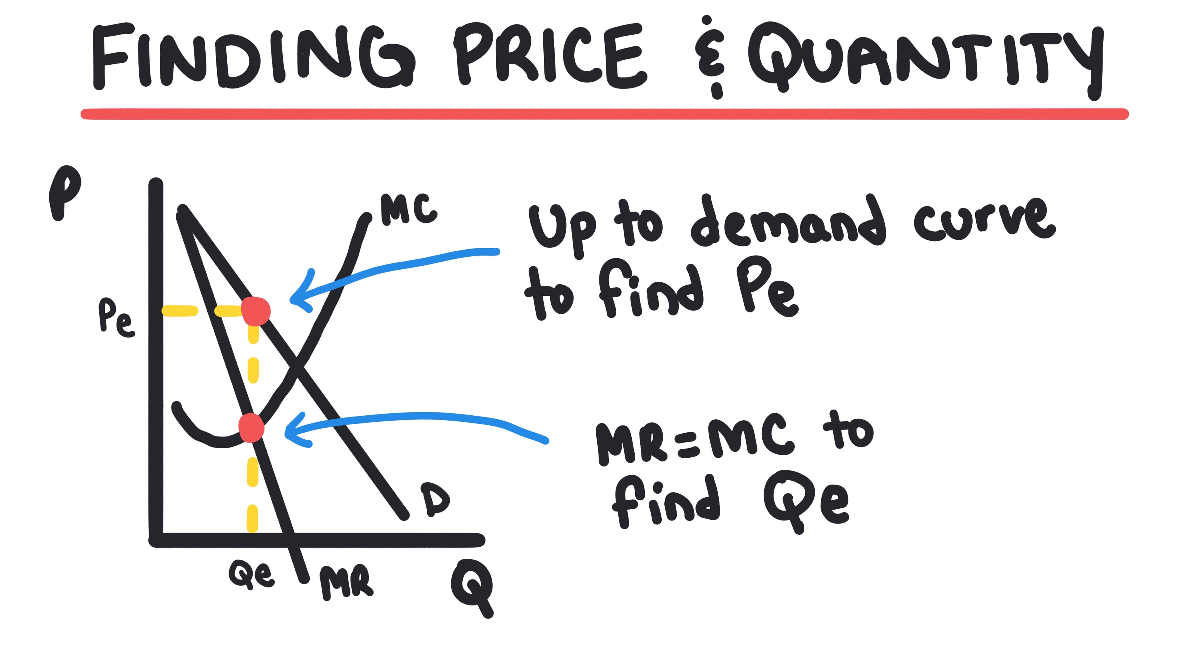
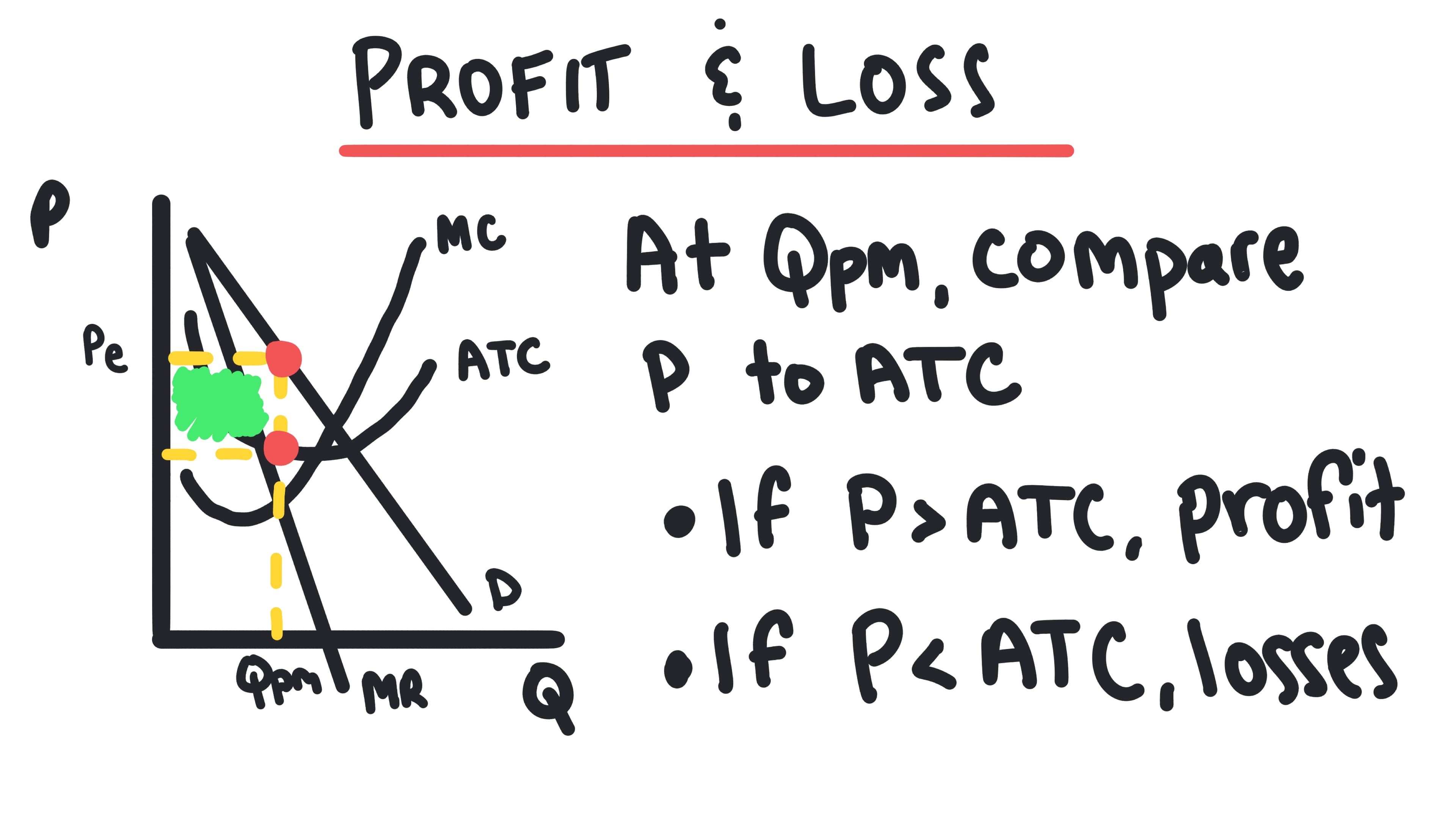
Profit Maximization Rule
To maximize profit (or minimize loss), a firm should produce the quantity where Marginal Revenue equals Marginal Cost.
- •Rule: Produce where MR = MC
- •When MR > MC, the firm earns additional profit (MR - MC > 0) for each additional unit produced, so it should continue producing more units.
- •When MR < MC, the firm loses profit by producing an additional unit, so it should reduce production.
- •Profit is maximized at MR = MC because the firm has produced all units where MR > MC (gaining profit) but has not produced any units where MR < MC (which would reduce profit).
Whiteboards
3.6 - Firms' Short-Run Decisions to Produce and Long-Run Decisions to Enter or Exit a Market
Key Terms & Definitions
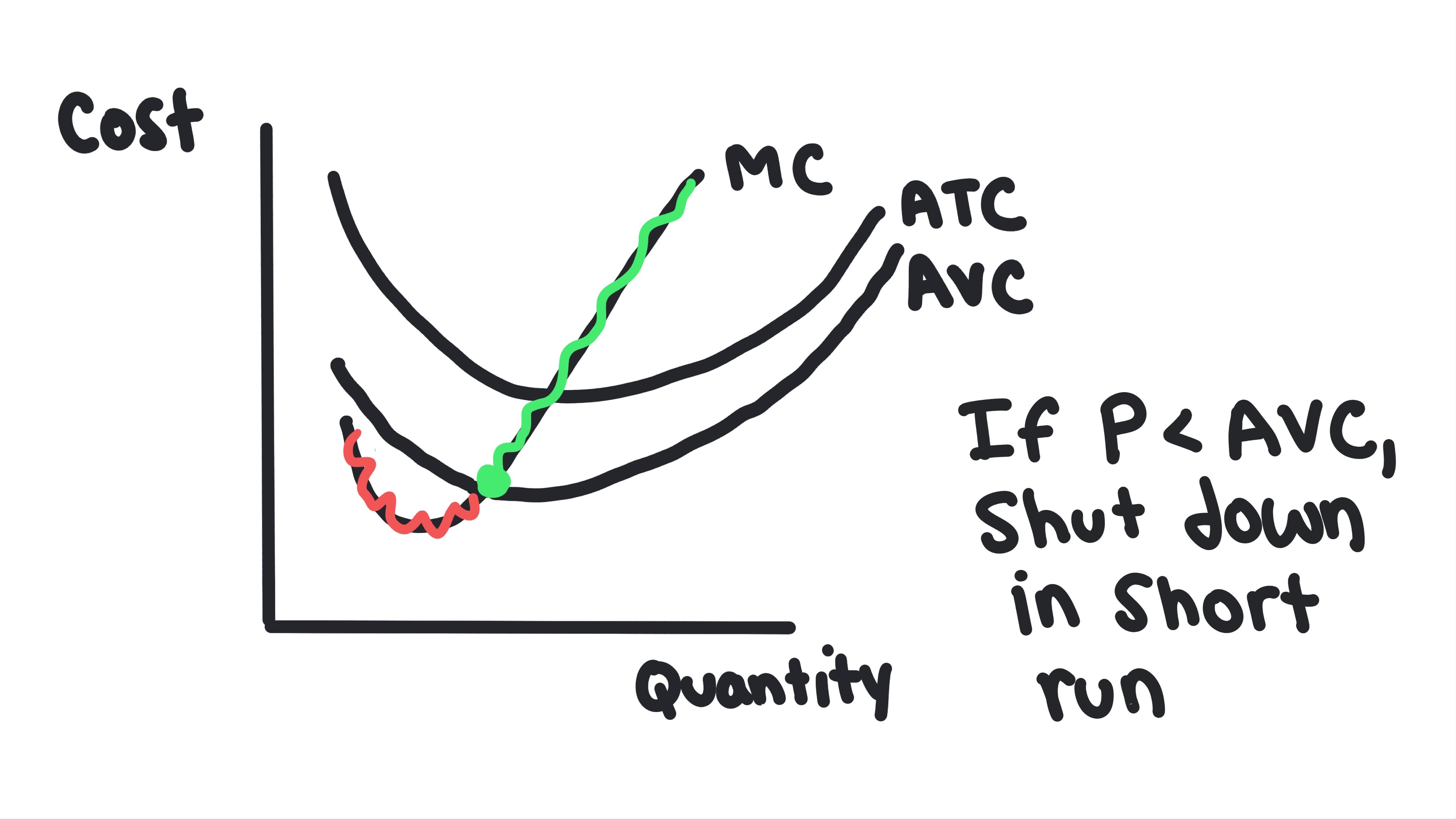
Shutdown Rule
In the short run, a firm should shut down (produce quantity zero) if the price falls below the minimum Average Variable Cost (AVC).
- •If P < AVC, the firm loses more by producing than by shutting down.
- •If P > AVC but P < ATC, the firm produces at a loss to cover some fixed costs.
Short-Run Supply Curve
For a perfectly competitive firm, the portion of the marginal cost curve that lies above the minimum average variable cost.
- •The firm will produce where P = MC, but only if P ≥ min AVC.
- •If P < min AVC, the firm shuts down and supplies zero output.
- •The market supply curve is the horizontal sum of all individual firm supply curves.
Barriers to Entry
Obstacles that prevent new firms from entering a market, such as patents, high start-up costs, or control of resources.
- •Perfect competition has NO barriers to entry (free entry and exit).
Whiteboards
3.7 - Perfect Competition
Key Terms & Definitions
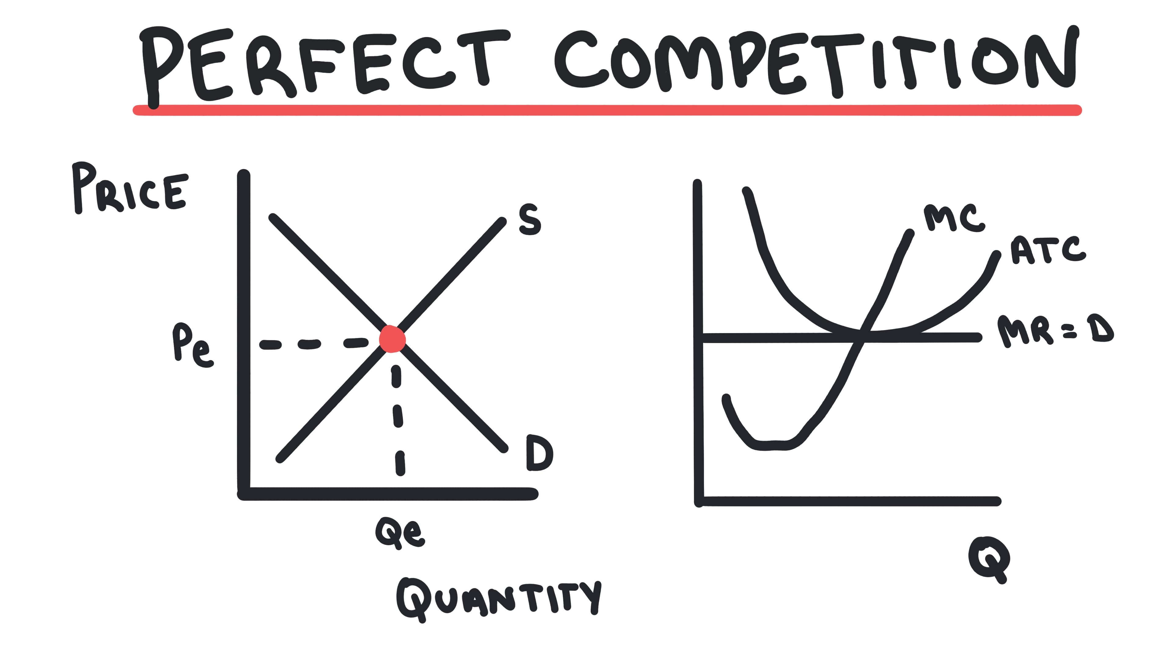
Characteristics of Perfect Competition
A market structure with many small firms, identical products, and easy entry/exit.
- •Firms are "Price Takers" (they cannot set their own price).
- •Demand for the individual firm is perfectly elastic (horizontal).
Perfectly Competitive Industry
An industry characterized by many firms, identical products, free entry and exit, and perfect information.
- •In the long run, firms enter when there are positive economic profits and exit when there are losses.
- •Entry and exit drive economic profit to zero in long-run equilibrium.
- •Examples include agricultural markets and stock exchanges.
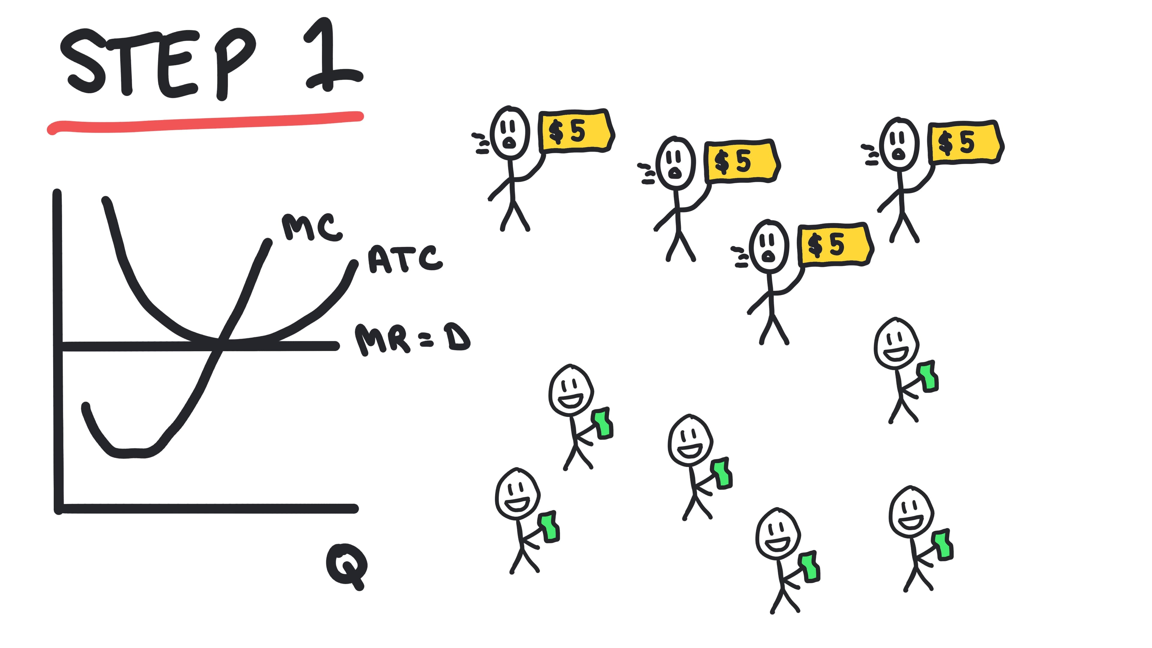
Positive Economic Profits
When total revenue exceeds total cost (including both explicit and implicit opportunity costs).
- •In perfect competition, positive economic profits attract new firms to enter the industry.
- •Entry increases supply, lowers price, and reduces profits until they reach zero.
- •Economic profit = Total Revenue - (Explicit Costs + Implicit Costs).
Mr. DARP
Acronym for the horizontal line facing a perfectly competitive firm.
- •Marginal Revenue = Demand = Average Revenue = Price
- •P = MR = AR = D
Long-Run Equilibrium (Perfect Competition)
The situation where firms enter or exit the market until economic profit is zero.
- •Price equals minimum ATC (Productive Efficiency).
- •Price equals MC (Allocative Efficiency).
- •No incentive for firms to enter or leave.
Productive Efficiency
Producing a good in the least costly way; producing at the minimum of the Average Total Cost (ATC) curve.
- •Perfectly competitive firms achieve this in the long run.
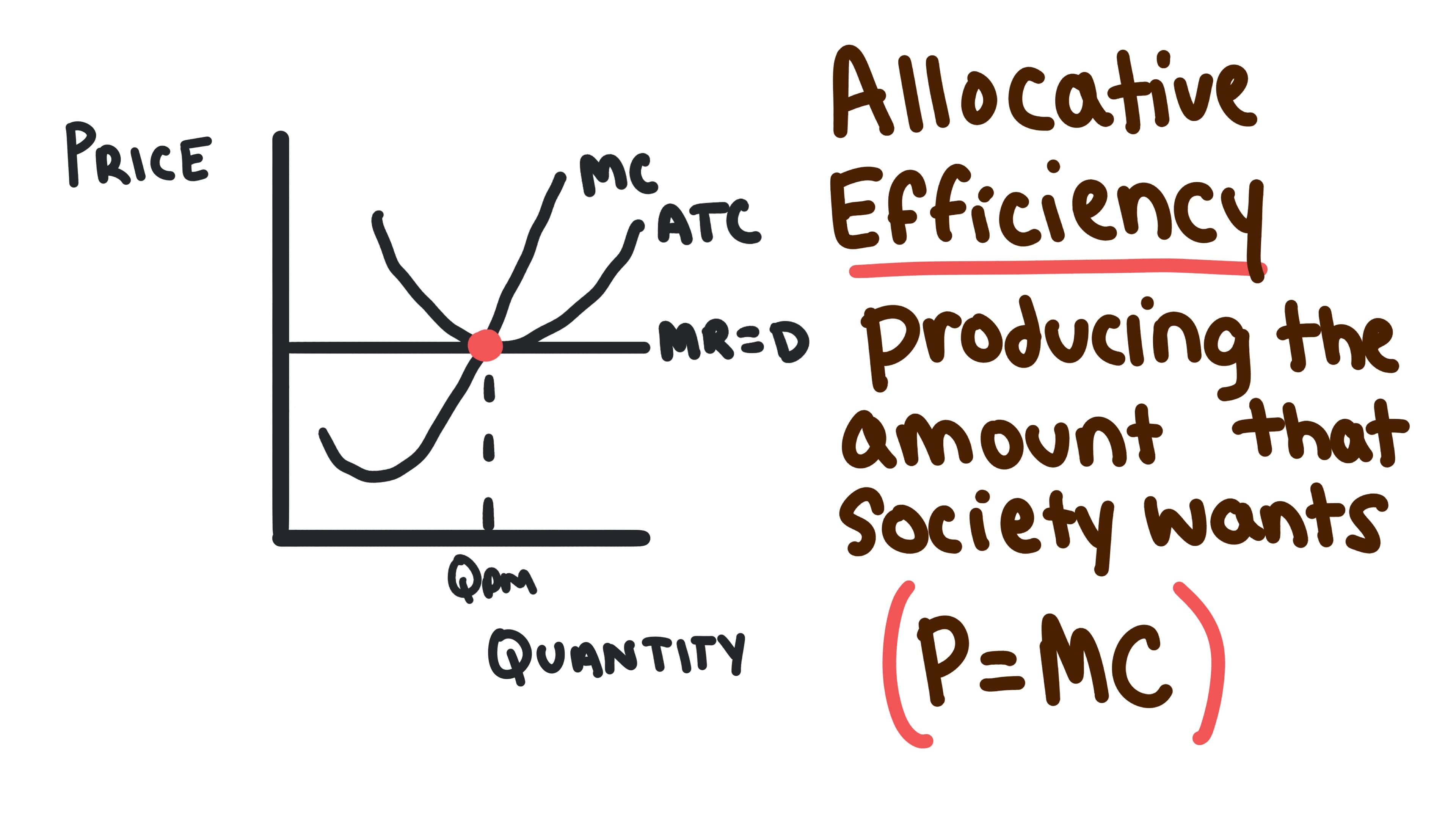
Allocative Efficiency
Producing the amount of goods that society most desires; producing where Price equals Marginal Cost (P = MC).
- •Perfectly competitive firms achieve this in both the short run and long run.
Whiteboards
Checkpoint
Test your understanding of 3.5
A profit-maximizing firm produces where:
Checkpoint
Test your understanding of 3.6
In the short run, a firm should shut down if: